Viscous Sphere

In this tutorial, we will run our first 3D case: steady low Reynolds number flow about a sphere using elements of order p=2. The root directory for this case is Tutorials/Steady_Sphere_Navier-Stokes.

Mesh Generation

The mesh generation for this case mirrors that of the 2D cases: we create a linear GMSH mesh and then generate a high-order mesh using MeshOpt. The geometry definition for this case is contained in the file Sphere25CSymmetry.stp. The GMSH configuration file for this tutorial, SphereSymmetry.geo, is duplicated below:

ff_len = 5;
max_lan = ff_len;
surf_len = 0.2;
dist = 10.0;
cuttof_dist = 1;


Mesh.CharacteristicLengthMax = ff_len;
Mesh.SaveParametric = 1;
Merge "Sphere25CSymmetry.stp";


Physical Surface(20) = {10};
Physical Surface(6) = {5:9};
Physical Surface(7) = {1:4};

Physical Volume(0) = {1};

Field[1] = Box;
Field[1].VOut = ff_len;
Field[1].VIn = surf_len;
Field[1].XMax = 1.0;
Field[1].XMin = -0.75;
Field[1].YMax = 0.75;
Field[1].YMin = -0.75;
Field[1].ZMax = 0.75;
Field[1].ZMin = -0.75;

Field[2] = Box;
Field[2].VOut = ff_len;
Field[2].VIn = 2*surf_len;
Field[2].XMax = 10;
Field[2].XMin = -1;
Field[2].YMax = 1;
Field[2].YMin = -1;
Field[2].ZMax = 1;
Field[2].ZMin = -1;

Field[3] = Box;
Field[3].VOut = ff_len;
Field[3].VIn = 4*surf_len;
Field[3].XMax = 30;
Field[3].XMin = -2;
Field[3].YMax = 2;
Field[3].YMin = -2;
Field[3].ZMax = 2;
Field[3].ZMin = -2;


Field[10] = Min;
Field[10].FieldsList = {1,2,3};

Background Field = 10;

There are some critical differences between this configuration file and those of the 2D cases. First, we specify boundary conditions on surfaces instead of lines, using GMSH's Physical Surface() command. We apply a no-slip boundary condition on the sphere surface (surfaces 1:4) and a far-field condition on surfaces 5:9. A symmetry condition is imposed on surface 10. Lastly, we must include Physical Volume(0) = {1}, otherwise GMSH will not write out all the elements.

Now that the we have a configuration file, it is time to create the GMSH mesh:

gmsh -3 -optimize -smooth 5 SphereSymmetry.geo

Note that we pass GMSH the -optimize command line argument. This tells GMSH to optimize the 3D mesh quality. It has no effect in 2D, thus it was left out of the previous tutorials.

The next step is to create the high order mesh using MeshOpt. The configuration file MeshOpt.config is shown below.

CaseParameters{
	GMSHFileName = SphereSymmetry.msh;
	STEPFileName = Sphere25CSymmetry.stp;
	OutputFileName = SphereSymmetryBL.msh;
}

BLParameters{
	GenerateBL = true;
	Thickness = 0.3;
	NLayers = 3;
}

HighOrderParameters{
	Order = 2;
	TargetMinQuality = 0.9;
	OptimizedNodeSpacing = true;
}

We generate the high order mesh, SphereSymmetryBL.msh, as before.

###Configuring and running the solver The configuration file for this case is:

Project{
	Name = Steady_Sphere;
	MeshFile = SphereSymmetryBL.msh;
	Equation = Navier-Stokes;
	Discretization = EDG;
	OptimizedNodeSpacing = true;
}

EquationParameters{
	gamma = 1.4;
	Pr = 0.72;
	Re = 40;
	M_inf = 0.2;	
	U_inf = {1,0,0};
}

NonlinearSolverParameters{
	RelTol = 1.0e-10;
	MaxIt = 100;
	Type = Quasi-Newton;
}

LinearSolverParameters{
	RelTol = 1.0e-4;
	Restart = 300;
	MaxIt = 300;
}

PostProcessingParameters{
	ValuesToSave = rho p M s |Vort|;
	NRefinements = 2;
}

Here, we select to use EDG instead of HDG, since it is more efficient for p < 4, especially in 3D. Note that for p=2, the optimized nodal interpolation points are identical to equispaced nodes. The Reynolds number is set to 40 and the Mach number to 0.2, with a unit velocity in the x direction. The other parameters are similar to what we have encountered in the previous tutorials.

Now we can run the case:

mpirun -np 4 FlowEDG

This example should require approximately 10 minutes of runtime using four MPI processes. It should be noted that this case does not converge if we increase the order to p=3. A more robust nonlinear solver is needed in such cases, featuring pseudo-time stepping and CFL ramping.

Post-Processing

As before, the results are post-processed with ParaView. Below we show an isosurface of Mach number colored by pressure.

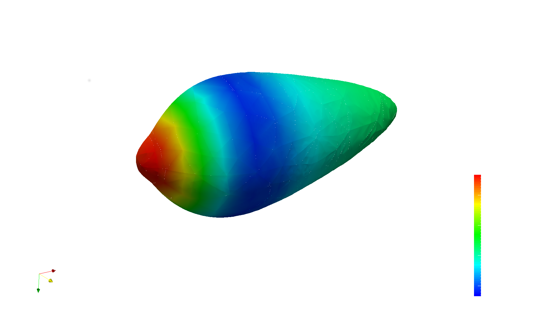
It is easy to see that this case is under-resolved. We are slowly working to improve the ability of FlowEDG to converge steady-state 3D cases, but our current priority is unsteady LES.