Methods
The primary need of the project was to either convert data and load it to the DPP street centerline (referred to as 'RCL' or Road Center Line in documentation), or calculate new data and load it to the RCL. The final data product was a single, "Modal Composite" dataset with numerous attributes. Ea
| Workflow Type | Automation Level | Explanation |
|---|---|---|
| Manual | None | Automation routines were evaluated but deemed to be not worth developing. Workflow was conducted manually.\ |
| Python Toolboxes | Semi/Fully Automated | Workflow uses custom Python Toolboxes. May consist of manual "QC" steps to validate outputs or select inputs to further analysis steps. All tools are loaded to ROW_tools.tbx |
| Jupyter Notebook | Fully Automated | Workflow runs as a standalone python developed in a Jupyter notebook environment. Workflow is intended to be run one cell at a time, modify as needed. |
Note: For workflows utilizing Jupyter Notebooks, technical documentation is located in the analysis notebook itself, with only reference links in this wiki.
The project analysis consisted of the following major steps. Some steps were performed in parallel by different team members. As new methods were developed, some steps were revised.
-
Convert 1986 ROW table to digital and load attributes to RCL. (Manual)
-
Estimate ROW width in GIS (referred to as '2020 ROW Estimate') as the distance from parcel-to-parcel across the street centerline. Load attributes to RCL. (Python Toolboxes)
-
Estimate on-street parking count using available GIS data. (Python Toolboxes)
Note: This data was not loaded to the final "Modal Composite" dataset as an attribute.
-
Load Pedestrian dataset attributes to RCL. Load Bike dataset attributes to RCL. (Jupyter)
-
Load attributes from 2020 ROW Estimate, 1986 ROW table, and TransCAD 2020 to the RCL. (Python Toolboxes)
Note: The process of loading TransCAD 2020 attributes to RCL necessitate the development of a modified spatial join workflow as the two datasets did not share geometry or attributes. This workflow, referred to as 'Custom Spatial Join' was used in different parts of the project to combine datasets with non-coincident geometry. Please see step 4b for mote details.
-
Develop Modal Width calculations for all modal attributes assembled to the RCL. (Jupyter)
-
Assign Complete Street Types to all street segments in RCL. Auto-assign using analysis logic. (Jupyter)
-
Revise Complete Street Types. Review and revision of typologies by DTS and project team. (Manual)
-
Develop and implement prioritization logic for Constrained Scenario. (Jupyter)
-
Perform additional spatial analysis related to Land Value, Sea Level Rise, and Economic Justice metrics. (Jupyter)
-
Create final summary metrics from Modal Composite Dataset. (Jupyter)
The 1986 ROW Table is a scanned PDF of a document created and formatted on a typewriter. The document contains street segment names and descriptions, planned and current right-of-way, number of lanes and other information about approximately 1000 road centerline segments on the island of Honolulu. This data was joined to Honolulu road centerlines to bring the historical data into the GIS.
Assumptions: None
Online Resources: None
Method: Manual
The 1986 ROW table is a PDF document created from a scan of the original document. The scan did not use optical character recognition (OCR), so the 1986 data is embedded into the document as a series of images.
The document was manually converted to a digital format by reviewing each item in the PDF and copying it to an excel document. Attempts at using OCR to convert the data, in conjunction with data clean up routines (python) created output that required manual intervention and review. This process, tested on a sample set of pages, proved to be more time intensive than manually converting the document and was thus abandoned in favor of manually recreating the original data tables.
The excel document created during the conversion process was imported into GIS using the ArcGIS Pro Excel to Table tool. The data table was then manually joined to road segments using the following steps:
-
Add a text field to the 1986 ROW Table in the GIS using the Add Field Tool.
-
Calculate that field to be equal to !objectid! + !Facility!.toUpper() using the ArcGIS Pro Calculate Field tool. For example, key value 11-LEHUA AVE signifies OID 11 and facility name Lehua Ave. This field represented the foreign key between the two datasets.
-
Remove any trailing periods from that field using the Calculate Field tool.
-
Add a text field to the road centerline data using the Add Field tool. This field is the primary key, or join field, between the two datasets.
-
Configure ArcGIS Pro to display the 1986 ROW table and the road centerlines. The analyst hid most fields in the road centerline data.
-
Select a series of road centerlines using the Select Layer by Attribute Tool. The analyst visually reviewed the selected features and used the selection tools (add to, remove from, create new and clear selection and keyboard shortcuts) to refine the selected road centerlines.
-
The analyst used the attributes pane in ArcGIS Pro to apply a single 1986 ROW Table OID+Facility ID value to all selected rows at once.
-
Finally, once all 969 rows from the 1986 ROW table were reviewed and their key value copied into the road centerline data, the GIS analyst formally joined the two datasets using the ArcGIS Pro Join Field tool. This moved attributes from the 1986 table to the road centerline data.
Use of the attribute pane, double clicking within the attribute table, accessing geoprocessing history to re-execute commands, changing selection tools and employing keyboard shortcuts enabled the analyst to rapidly enter all 1986 ROW Table values into the road centerline data.
Once this was complete, another team of analysts reviewed a sample of the data to verify correctness and visited all records that could not be initially matched manually by the GIS analyst. Once this review was complete, findings were returned to the GIS analyst, who made corrections and updated rows.
Converting a legacy document into modern digital content is challenging. As the original document was formatted on a typewriter, optical character recognition was not effective. Also, the scanned document had watermarks which further foiled the OCR operation. However, there were only 969 elements from the document to process, so the manual conversion and manual entry into the GIS were not difficult. Furthermore, ArcGIS Pro is a mature production tool that enables easy and rapid editing.
The potential improvement with the greatest impact would be to further research OCR tools to convert the legacy PDF document more effectively and rapidly into modern content usable across multiple platforms. The only OCR tool used was Adobe Acrobat. While it was effective, output was not good enough to be used without significant manual intervention. It’s likely that a machine learning approach could have produced a better outcome.
Right of way was estimated as the distance between parcels that are separated by a road centerline. The estimation was done in the GIS using ArcGIS Pro and Python Script tools to wrap and control geoprocessing tool behavior.
- ROW is the distance between parcels that are separated by a road centerline.
- ROW is estimated as the min, max and average distance between parcels separated by a road centerline, along a road centerline segment.
Online Resources: https://github.com/Ray-Mangan/DTS-Complete-Streets/blob/main/ROW%20Tools.tbx
Method: Python Toolboxes
ROW estimation was divided into three phases:
-
Data prep - Step in which data was progressively thinned to improve analysis processing.
-
Data processing – Step in which ROW Distance analysis was executed. ROW was estimated, in this case, as the distance between parcels separated by a road centerline. Output is a table and feature class with min, max and mean ROW distance per RCL.
-
Results analysis – Step in which outputs were analyzed for validity, accuracy and completeness.
Data Prep
In this phase, supporting datasets were progressively thinned to remove unneeded rows from the analysis. This enabled faster processing and more accurate estimation.
The following table details the spatial operations employed to reduce the amount of data pushed through the ROW estimation analysis.
| Action | Description |
|---|---|
| Filter out H1, H2, H3 from RCLs | Highways not needed in analysis |
| Erase parcels on federal lands | Remove bases and other fed lands from processing |
| Erase RCLs on federal lands | Remove roads in bases and other fed lands from processing |
| Erase parcels on Hawaiian Homelands | Remove HHLs from processing |
| Erase RCLs on Hawaiian Homelands | Remove roads in HHLs from processing |
| Erase parcels on State Parks | Remove parcels within state parks from processing |
| Erase RCLs in State Parks | Remove roads in parcels within state parks from processing |
| Remove Street Parcels | Remove roadway deeds that were never transferred to the City |
| Erase RCLs within roadway deed parcels | ROW = distance between parcels separated by an RCL |
| Delete short RCLs | Remove RCLs with a shape length < 50 |
The table above references datasets that were used to erase road centerlines and parcels.
The following table categorizes these datasets as constraints layers and lists their sources:
| Constraints Layer | Source |
|---|---|
| Federal lands | https://honolulu-cchnl.opendata.arcgis.com/datasets/federal-owned-land |
| Hawaiian homelands | https://dhhl.hawaii.gov/po/maps/ |
| State and local parks | https://geoportal.hawaii.gov/datasets/parks-polygons-kauai-oahu-maui |
Data Processing The Data Processing phase covered the effort to estimate the distances between parcels that are separated by a road centerline. As these distances can vary along a road centerline, sampling and distance measuring techniques were developed to generate an estimate of minimum, maximum, and average ROW along a road centerline.
Custom python script tools were used to generate the ROW distances. The following process was used to estimate ROW:
-
Find the closest parcel feature to each road centerline.
-
Script tool, 01_Create Near Points, generates a point every 50’ along each RCL.
-
The script tool runs the Near Geoprocessing tool to locate the closest parcel from each point. This process enables a sampling of closest parcels along each RCL.
-
The script tool creates a dataset that indicates the closest location on a parcel edge to the sampling point.
-
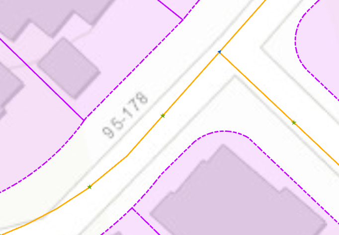
In the graphic below, the green starts represent a 50’ increment along the yellow road centerline. The purple shapes are parcels. This is the output of Create Near Points.
-
-
Find the closest opposite parcel from the near parcels identified in step 1:
-
Script tool 02_Generate Opposite Near Parcel Points uses the NEAR_X and NEAR_Y information from step 1 to find an angle from the points along the RCLs to the closest parcel edge.
-
The tool reverses that angle by adding or subtracting 180 degrees.
-
The tool adds NEAR_DIST to an offset value to create a new point.
-
A 60’ offset factor was used for processing.
-
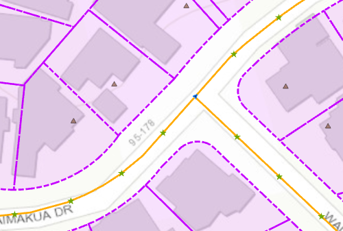
In the graphic below, brown triangles are generated by reversing the angle between the green stars and the NEAR_X and NEAR_Y values associated with each green star. A new point is created at angle and a distance of NEAR_DIST + offset factor.
-
-
Find which of points created by step 2 are within (and not within) parcels.
- Custom script tool, 03_Intersect Points With Search Areas, selects points within parcels and then reverses the selection to select points outside the parcels.
- The tool writes each selection set to a new output dataset.
- Points not within parcels can be used to rerun Generate Opposite Near Parcel Points with a larger offset to locate parcels.
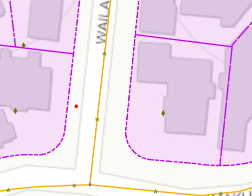
- The graphic below displays dark green diamonds that represent output points within parcels. Red boxes represent points outside of parcel.
-
Estimate ROW distances:
- Script tool 04_Make Connection Lines for Intersection creates a line between each point created by step 3, its original sampled point on the road centerlines, and the NEAR_X and NEAR_Y values in that sampled point.
- The tool intersects that line with parcels
- The tool generates a new line from an intersected parcel edge to the parcel edge indicated in the NEAR_X and NEAR_Y fields.
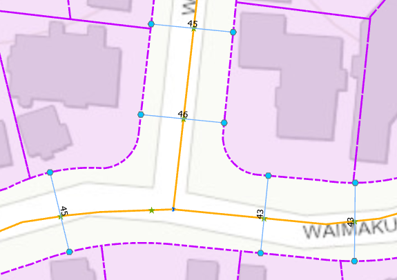
- The graphic below displays blue lines that represent the distance from parcel edge to parcel edge. This distance is the estimated ROW width at a sampling point location. The blue lines are labeled in feet (and rounded). Rounding is only applied to displayed values, not database values.
-
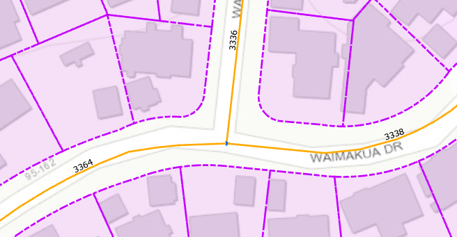
Estimate the row distances for each RCL SegmentID:
- Script tool, 05_Summarize ROW Distances, summarizes each connection line created in step 4 by SegmentID.
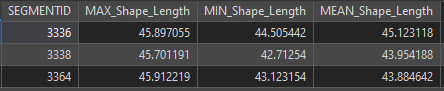
- The script tool generates max, min and mean distances per SegmentID.
- In first graphic below, orange RCLs are labeled with their associated SegmentID values.
The second graphic shows each SegementID’s max, min, and mean ROW estimate values.
Results Analysis Key analysis results include the following:
- The data prep stage removed 8505 (out of 27062) road centerlines from the analysis. 18554 road centerlines were used in the analysis.
- The data prep stage removed 5389 parcels (out of 170721) parcels from the analysis. 165446 parcels were used in the analysis.
- Total number of segments (road centerlines) for which ROW was estimated: 16742.
- Total number of segments (road centerlines) for which ROW could not be estimated: 1812. This equated to 9.8% of segments used in the analysis and 6.7% of total segments. These values represent the number of RCLs that could not generate a ROW. This is due to the distance to an opposite parcel exceeds NEAR_DIST + 60’. This equates to the max search distance for a parcel from a specific point.
- The number of points generated by the tools that do not fall within a parcel was 26392. Of the 26392 points that did not land in a parcel, 4738 are within 10’ of a parcel. This difference accounts for 3% of the analysis.
Subsequent analyses should consider the following:
- The data prep stage removed parcels that could have been used in the analysis. Parcels comprising military bases, etc, could form boundaries useful to the analysis, especially for the number of search points that did not fall within a parcel. A visual inspection, conducted post-processing, would reveal which parcels to include. This does not apply to all removed (thinned) parcels.
- Increasing the search distance (NEAR_DIST + 60’) could also increase the estimation accuracy. Slight increases should be tested first (70’, 80’, 90’). Increasing the search distance too much will result in false positives.
- The initial sampling distance used in Create Near Points was 50’. Subsequent runs could use smaller distances. This might increase estimation accuracy. Decreases to this distance should be accompanied by adjustments to the Data Prep stage step Delete short RCLs.
Total on-street parking for the island was estimated for each road centerline segment and summarized by traffic analysis zone on the island of Honolulu. Analysis was done using a series of python script tools in ArcGIS Pro.
- Use conventional spatial analysis tools
- Rapidly generate an estimate
- Use multiple city and county data sources to perform estimate
- Parking Specific Assumptions:
- If a segment has metered parking, then no on-street non-metered parking is allowed along that segment
- On-street parking stalls are 20’
- No parking zone on 15' on either side of a hydrant
- No parking zone within a 100' around a bus stop
- No parking zone within an 18' area per driveway
- No parking zone within 50' of an intersection along an avenue, parkway or a boulevard and within 20' of an intersection along any other street type
Online Resources: https://github.com/Ray-Mangan/DTS-Complete-Streets/blob/main/ROW%20Tools.tbx
Method: Python Toolboxes
The on-street parking estimate employed conventional spatial analysis tools to rapidly generate an estimate per City and County of Honolulu road centerline SegmentID and traffic analysis zone (TAZ). A GIS Analyst created an ArcGIS Pro Toolbox with 6 script tools to perform this spatial analysis. Work was spread across 6 tools to enable QC of each step. All outputs from the tools are derived to reduce clicks across analysis runs.
On-street parking was estimated per SegmentID using the following process:
- Erase RCLs from agriculture and conservation land use types.
- Filter out street types: EXIT; FWY; HWY; ON RAMP; RAMP.
- Filter out TIGER classes: A71; A64; empty or null.
- NEAR + JOIN FIELD RCLs to hydrants, bus stops and buildings to estimate the number of hydrants, bus stops and buildings (driveways) per SegmentID. The tool counts each building as having 1 driveway. This causes an undercount as many buildings share or have not driveways.
- Intersect RCLs on RCLs to generate points where RCLs cross.
- Spatial Join RCLs to the intersection points to find the number of intersections per SegmentID.
- Remove SegmentIDs that already have metered parking associated to them.
- Remove SegmentIDs that have protected bike lanes along them. Protected bike lane is a type.
- Spatial Join RCLs to the PED plan to process the Roadway Buffer attributes (SB and NB).
- If SB or NB roadway buffer = 0,1 or 1,0, reduce the number of driveways by 50% as there's only 1 side available for parking.
- Create a no parking zone on 15' on either side of a hydrant.
- Create a no parking zone within a 100' around a bus stop.
- Create a no parking zone within an 18' area per driveway.
- Create a no parking zone within 50' of an intersection along an avenue, parkway or a boulevard and within 20' of an intersection along any other street type. Multiply the value by 2 (to account for both sides of the street) under the following conditions:
- SB and NB = null
- SB and NB = 1
- SB and NB = 0
- For each segmentID, subtract the total no parking space from the segmentID length, then divide by stall length (20'). This is the estimate of the number of spaces per segmentID.
- If SB and NB = 1, multiply the total by 2 to account for space on either side of the street. Summarize the segmentIDs within each TAZ, summing the number of stalls per segmentID. This generates the total stalls per TAZ.
The method detailed above provided a quick, rough-order-of-magnitude estimation. However, several improvements could be made to improve the accuracy of the estimate.
Improvement #1 Use machine learning and feature extraction to supplement existing datasets. One of the analysis assumptions no parking zone within an 18' area per driveway distorted the estimate. Driveway data was incomplete or missing so there was no accurate way of identifying the location of the driveways. The analysis assumed that each building would have a driveway. This is incorrect as there are many buildings on the island that do not have driveways (clusters of apartment buildings, city blocks, etc). Using the higher quality imagery available on the island, the ArcGIS Pro machine learning analytical modules could have been employed to extract driveways. With that information, a more accurate estimate would have been performed.
Improvement #2 Tightly define rules for the ped plan dataset. The ped plan data was used to incorporate segments with a protected bike lane. The ped plan is not as complete as the road centerline data, creating null values in the following conditions: • Spatial join between the road centerlines and ped plan where there were no ped plan features • Ped plan SB or NB roadway buffer is null The SB and NB roadway buffer attribute was used in the parking estimate. Ideas for handling ped plan nulls were discussed after the initial estimate was complete when it was realized that nulls were distorting the analysis. The following ideas were discussed but never explored due to budget constraints: • Consider features that are not part of the ped plan as unimproved streets. • Unimproved streets have no curb or gutter (asphalt and grass) and the ped plan has a curb attribute. If there’s a curb, it’s an improved street. • Null values will have no ped plan data, apply a ratio or rule for these spaces. • Examine the additional attribute and if there’s no value, exclude the segment.
Improvement #3 Further testing of the final calculation of stalls in python script tool CalcStallsPerStreet is needed.
functionDef = """
def calcStalls(sb, nb, rclLen, intOffset, hydrants, stops, dwys, hydrantSpace, busSpace, dwySpace, stallSpace):
    if (sb == 0 and nb == 1) or (sb==1 and nb == 0):
        return lenWithNoPKing / stallSpace
    else:
        return (lenWithNoPKing *2) / stallSpace """
This function is used in the script tool and passed to the ArcGIS Pro Field Calculator tool. There are some cases in which the output value is negative. Negative values are ignored later in the script. Further refinement of this was postponed due to budget constraints.
Compile fields from DTS Sidewalk Inventory, Proposed Sidewalk Improvements, Proposed Sidewalk Additions, Current Bike Facilities, Proposed Bike Facilities, and Redevelopment Bike Facilities to DPP Street Centerline feature class. Datasets are compiled together either by directly joining on SegmentID, or by performing an Intersect, then joining the output using SegmentID
Assumptions: (see Jupyter Notebook) Online Resources: https://github.com/Ray-Mangan/DTS-Complete-Streets/blob/main/DTS%20-%2004%20-%20Modal%20Composite.ipynb Method: Jupyter
(see jupyter notebook)
(see jupyter notebook)
Previously steps created a modal composite dataset with attributes from the Ped and Bike plans. The next phase was to incorporate TransCAD information into the Modal Composite dataset.
Assumptions: None
Online Resources: https://github.com/Ray-Mangan/DTS-Complete-Streets/blob/main/ROW%20Tools.tbx
Method: Python Toolboxes - "Custom Spatial Join" Script Tool
The traditional method to incorporate attributes (information) from one dataset to another is to use a Join. Joins in GIS can be done on a common key using traditional relational database methodology, or spatially using different tools based on spatial relationships. There must be a relationship between dataset rows or geometries for a join to be successful.
Joining the TransCAD to Modal Composite datasets involved the following challenges:
-
There is no common field between the TransCADand Modal Composite datasets so they cannot be joined using traditional table joins or using the ArcGIS Pro Join Field tool.
-
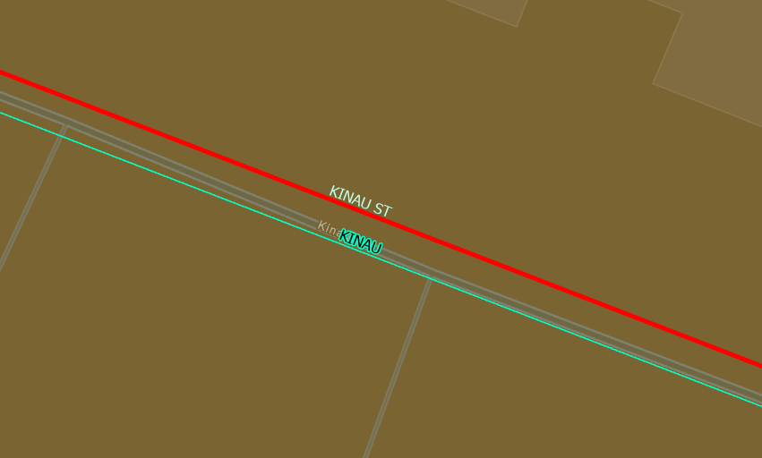
The TransCAD features are not spatially coincident with the Modal Composite features. This means that although both datasets model the same roads on the island of Honolulu, they do not have a shared geometry. Since they are not coincident, a simple spatial join is not enough to join attributes from one dataset to the other. While both datasets overlap and intersect, they do not do so consistently. This makes manual editing using snapping and other editing rules onerous, slow, and expensive.
In the example graphic below, the red line represents the TransCAD 2000 data and the green line represents the modal composite data. Both lines are Kinau St. In this example, the lines are approximately 7’ apart.
-
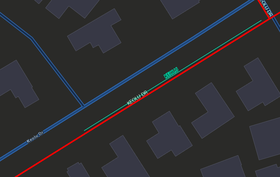
TransCAD features do not equate, in length, to Modal Composite features. This means that a TransCAD feature may be longer, shorter or close to the same size. This prevents other simple spatial join operations, including Spatial Join, Near and Buffer from providing a quick and easy solution. It also causes ambiguity in the join between the two datasets. For example, in the following graphic, the red feature represents Keolu Dr and the green feature represents a Segment along Keolu Dr. Notice how the red line extends far beyond the Segment. When these two datasets are joined so that attributes from TransCAD are transferred to the Segment, there is ambiguity as to which Segment should get those attributes since the lines do not match.
To successfully join the two datasets so that attributes from TransCAD are transferred to road centerline segment geometries, the following process was created and executed as a python script tool in ArcGIS Pro:
- Intersect the input TransCAD data w/the modal composite layer to create intersection points where the two datasets cross. Dissolve the output to remove any coincident intersection points.
- Intersect the modal composite layer with itself to create intersection where the dataset crosses itself. Again, dissolve the output to remove any coincident intersection points.
- Combine the two datasets created in steps 1-2 into a single dataset.
- Buffer, by 25’, the single dataset created in step 3 to create.
- Erase, using the buffer generated in step 4, parts of segments from the modal composite dataset. This creates distance between the modal composite dataset and the TransCAD data. This distance prevents subsequent spatial joins from picking up false positives around intersections.
- Buffer the TransCAD data to create search shapes. The search shapes are used to select modal composite features. The buffer distance used in this step is an input to the model and is therefore configurable.
Further refinement of workflow to catch edge cases (small line segments). Develop & train machine learning model if warranted to assist with repeated future workflows.
Utilize all previously compiled attributes in modal composite 05 in conjunction with standardized width parameters for elements in the street cross section to calculate Unconstrained Modal Width, Area, and other metrics.
Assumptions: (see Jupyter Notebook) Online Resources: https://github.com/Ray-Mangan/DTS-Complete-Streets/blob/main/DTS%20-%2005%20-%20Modal%20Widths.ipynb Method: Jupyter
(see Jupyter notebook)
(see Jupyter notebook)
Assumptions: (see Jupyter Notebook) Online Resources: https://github.com/Ray-Mangan/DTS-Complete-Streets/blob/main/DTS%20-%2006%20-%20Street%20Typologies.ipynb Method: Jupyter
(see Jupyter notebook)
(see Jupyter notebook)
After initial assignment of Complete Street Typologies, data was published to ArcGIS Online for review by DTS Staff. DTS Staff provided input on individual streets that were mis-assigned. Input was provided in the form of an ArcGIS Online point feature service, configured for editing by DTS staff with options to select a street type "override". Points were placed on the map on streets that needed adjustment.
Assumptions: (see Jupyter Notebook) Online Resources: https://github.com/Ray-Mangan/DTS-Complete-Streets/blob/main/DTS%20-%2007%20-%20Street%20Typology%20Overrides.ipynb
Method: Jupyter with additional Manual processing
(see Jupyter notebook)
(see Jupyter notebook)
Implement Modal Prioritization logic for street segments that have Unconstrained Modal Width > ROW Width estimate.
Assumptions: (see Jupyter Notebook) Online Resources: https://github.com/Ray-Mangan/DTS-Complete-Streets/blob/main/DTS%20-%2008%20-%20Modal%20Prioritization.ipynb Method: Jupyter
(see Jupyter notebook)
(see Jupyter notebook)
Calculate metrics related to Economic Justice and Sea Level Rise Exposure Area
Assumptions: (see Jupyter Notebook) Online Resources: https://github.com/Ray-Mangan/DTS-Complete-Streets/blob/main/DTS%20-%2009%20-%20Environmental%20Analysis.ipynb Method: Jupyter
(see Jupyter notebook)
(see Jupyter notebook)
Summarizes analysis results into key metrics for final report. This script utilizes in-memory data frames from the Pandas data science library for various calculations. Data frames have the benefit of loading the source dataset into memory for analysis, without modifying the source date.
Assumptions: (see Jupyter Notebook) Online Resources: https://github.com/Ray-Mangan/DTS-Complete-Streets/blob/main/DTS%20-%2010%20-%20Results%20Summary.ipynb Method: Jupyter
(see jupyter notebook)
(see jupyter notebook)