
Microsatellite Parameterized Analysis Tools
MicroSPAT is a collection of tools for semi-automated analysis of raw capillary electrophoresis (CE) data output by the ABI 3730. MicroSPAT integrates several features including a plate view for quality checking, automated ladder identification, sample based association of FSA data to keep data organized in a logical manner, automated bin generation using a clustering algorithm, automated artifact estimator generation, automated quantification bias estimation, and automated genotyping of samples with the option of manual curation. If you're using MicroSPAT, please Star the repo so that I know it is of use to people and I will continue development.
Under Very Heavy Development -- Features will change, things WILL break
Download the latest build zip, unzip, and navigate to the folder. Using either pip or conda, install the required packages either through requirements.txt or using the conda environment manager and the environment.yml file.
pip install -r requirements.txt
conda env create -f environment.yml
source activate microspat
If you plan to install through pip, I highly suggest using an environment manager, but this is beyond the scope of this tutorial. Once all packages are installed, execute the following
python manage.py initDB
This initializes the application with the HDROX400 Ladder
While in the MicroSPAT directory, execute the following
python manage.py runsockets
Then open Chrome (Only tested in Chrome to date, no guarantee for other browsers at this time) and navigate to:
http://localhost:5000
This will bring up MicroSPAT for the first time. At this point, you can then start to populate the application with your data.
The primary tools in MicroSPAT consist of 3 steps:
- Scanning the signal to find peaks
- Filtering out peaks that fit some criteria
- Analyzing the remaining peaks in a context dependent manner
The parameters used in scanning and filtering are common across most contexts, and individual projects will have further analysis settings that are more specific. The following is an explanation of the Scanning and Filter Parameters.
Scanning Parameters control the initial identification and coarse filtering of peaks. This is the most time intensive step, so these settings should not be changed if it can be avoided.
| Parameter | Description |
|---|---|
| Maxima Window | Final filter to remove close peaks. For each peak identified, take only largets peaks that fall within window size of each other |
There are currently two different algorithms available for use to determine peaks, Relative Maximum and Continuous Wavelet Transform. Relative Maximum is a fast simple algorithm that finds local maxima by sliding a window across the data and determining the maximum point within that window, thus identifying a peak. The data is first smoothed with a Savitzky-Golay filter and baseline corrected using a white-tophat transform before the Relative Maximum algorithm is applied. Continuous Wavelet Transform is a more complicated algorithm that works by convolving the signal with a series of wavelets from a given set of widths, and then determines peaks that appear at enough length scales and have sufficiently high SNR. In general, Relative Maximum is faster and typically works well enough, although a properly tuned CWT can perform very well in noisy data. More information can be found here http://bioinformatics.oxfordjournals.org/content/22/17/2059.long
| Parameter | Description |
|---|---|
| Relative Maximum Window | Number of points on each side of prospective peak to identify relative maximum |
| Smoothing Window | Window size passed to the Savitzky-Golay filter |
| Smoothing Order | Order of the polynomial used in the Savitzky-Golay filter to smooth the data |
| Tophat Factor | Size Factor to apply the white-tophat filter. Tophat filter footprint size is (Tophat Factor)*(length(signal)) |
| Parameter | Description |
|---|---|
| CWT Min Width | Minimum expected peak width |
| CWT Max Width | Maximum expected peak width |
| Min Signal to Noise Ratio | Min SNR, The signal is the value of the cwt matrix at the shortest length scale, the noise is the noise percentile of datapoints contained within a window around the identified signal |
| Noise Percentile | Used in Min SNR calculation |
| Gap Threshold | A ridge line is discontinued if there are more than Gap Threshold points without connecting a new relative maximum. |
Filter Parameters provide more nuanced filtering of peaks. This is fast, allowing for quick iteration on peak identification without having to rescan the signal for peaks.
| Parameter | Description |
|---|---|
| Min Peak Height | Peaks with peak height lower than Min Peak Height are filtered out |
| Max Peak Height | Peaks with peak height greater than Max Peak Height are filtered out |
| Min Peak Height Ratio | Secondary peaks with a height ratio compared to the primary peak less than Min Peak Height Ratio are filtered out |
| Max Bleedthrough Ratio | Let signal strength be the sum of the signal from -1 to +1 indices of a peak. Bleedthrough ratio is defined as the peak signal strength divided by the maximum signal strength of other channels in the same well at the same peak index. Peaks with a bleedthrough ratio greater than Max Bleedthrough Ratio are filtered out |
| Max Crosstalk Ratio | Crosstalk ratio is defined as the peak signal strength divided by the maximum signal strength of other channels in the same color in surrounding wells (surrounding wells defined as surrounding capillaries as they feed into the machine, not surrounding wells within the plate.) |
| Min Peak Distance | Peaks that are less than Min Peak Distance away (in nucleotides) are filtered out, leaving only the tallest peaks |
Ladders are the collection of settings that are used to identify ladder peaks in a well and then map the signal from the time domain to the base size domain, providing the base size of a given peak. MicroSPAT currently only provides a cubic spline interpolation method that generates a sizing quality metric which is essentially the weighted sum of squared residuals of the spline approximation.
Navigate to the Ladders tab on the left side. Populate the fields to the right with relevant information. At a minimum provide a unique label, a comma separated list of the base sizes of expected peaks, and the color of the dye used for this ladder. Scanning Parameters may be manipulated to affect how peaks are initially identified during ladder deterimination.
| Parameter | Description |
|---|---|
| Label | The unique label to identify ladder settings |
| Bases (Comma Separated) | Comma separated list of expected base sizes for peaks in ladder |
| SQ Flagging Limit | Maximum Sizing Quality value allowed before flagging a well as having a ladder sizing issue |
| SQ Unusable Limit | Maximum Sizing Quality value allowed before completely ignoring a well for downstream processing |
| Base Size Precision | Precision after decimal point for interpolating base size. In general does not need to exceed 2 |
| Index Overlap | Minimum number of data points between peaks, used for culling out false peaks and stutter in ladder determination |
| Min. Run Time | Discard data points before this value, used for culling out false peaks from beginning of run |
| Max. Peak Height | Remove peaks found to be greater than Max. Peak Height, used for removing outlier peaks due to bleedthrough from other channels |
| Min. Peak Height | Remove peaks found to be less than Min. Peak Height, used for removing outlier peaks attributable to low level noise and bleedthrough from other channels |
| Outlier Limit | Cull peaks that are outliers by height until only a set of peaks of length Bases + Outlier Limit exists, then use iterative algorithm to determine best fit curve to interpolate base sizes |
| Maximum Missing Peak Count | Maximum number of peaks that may be missing before ladder interpolation fails |
| Remove Outliers | Remove outliers in initial pass before applying iterative algorithm (Setting to true is in general faster) |
| Allow Bleedthrough | True => Keep peaks even if potential bleedthrough detected, False => Remove peaks where potential bleedthrough detected (Set to false if having issues with bleedthrough peaks being detected as real peaks) |
| Color | The color of the channel used for the ladder |
Loci represent discrete microsatellite regions in DNA, detected by amplifying specific fluorophore tagged primers. In MicroSPAT they are the settings that determine the base size range to look for alleles, the color they are tagged with, and the expected nucleotide repeat unit.
Navigate to the Locus tab on the left side. Populate the relevant information in the panel and press save to save the new locus. Label must be unique for every locus.
| Parameter | Description |
|---|---|
| Label | Unique label to identify locus |
| Min. Base Length | Minimum base size to identify alleles |
| Max. Base Length | Maximum base size to identify alleles |
| Nucleotide Repeat Length | Expected repeat unit of microsatellite locus |
| Color | Color of dye that locus will be labeled with. Must be one of (Red, Green, Yellow, Blue, Orange) |
You may load several loci all at once by uploading a csv file with a header containing [Label, Min. Base Length, Max. Base Length, Nucleotide Repeat Length, Color] and where each row is a new locus entry. A demo file is located at demo_files/load_loci.csv
All analysis in MicroSPAT revolves around Locus Sets. A locus set is a predetermined set of loci that you wish to analyze together. Every project is assigned a locus set and is used to determine the relevant run data for that project. This allows for analysis of different sets of loci in different contexts.
To create a new locus set, navigate to the Locus Sets tab on the left side. Create a unique label for the locus set, and select the loci to be in the locus set by clicking each row. Active loci will be highlighted green. Once all loci are chosen, press save at the bottom and the locus set will be added to the locus set pane.
Controls are sets of alleles that have been associated with a known sample. They are used to determine Quantification Bias Factors and in the future will be integrated into automated positive control QA metrics.
To register a control, there must first exist a valid Bin Estimator Project. Once a Bin Estimator has been created, navigate to the Controls tab in the left panel. Enter in a unique barcode for the control, select the appropriate Bin Estimator, populate the allele present for each locus, and press save.
All CE data must be uploaded into MicroSPAT in the "Plate Format", essentially all the FSA files that were created from a single CE run zipped together into a single zip file (96 FSA files in a 96 format run, 384 FSA files in a 384 format run)
To upload the plate, select "choose files" and select the zip. Next select the ladder used on this plate. At this point in time, MicroSPAT only supports one ladder on a plate. Press upload and MicroSPAT will process the plate, add it to the database, and calculate the ladder for each well. Multiple Plate zips may be uploaded at once and processed in parallel if they are all selected in the "choose file" prompt. Once complete the plate(s) will appear in the list below and an active plate will be shown to the right.
After a plate has been uploaded, a Plate Map may be used to assign each channel to a particular sample for a given locus. A Plate Map is a CSV file containing the assignment of each well to a particular sample and marker. The header will be [Well, locus1, locus2, ...] where [locus1, locus2, ...] are the unique labels of the loci that were run on this plate. Each row then contains the well and the samples contained for each marker. Ex:
| Well | L1 | L2 | L3 |
|---|---|---|---|
| A01 | P1-Sample1 | P1-Sample1 | P1-Sample1 |
| ... | ... | ... | ... |
A demo file showing how a plate where different markers are used in different wells can be found at demo_files/96_well_plate_map.csv. In order to upload a Plate Map, select a plate, and in the right pane press "Choose File" to select the Plate Map CSV. If you are adding new samples, select "Create Samples If They Don't Exist" to add new samples to the database. Note: Any new samples containing 'NTC' will be negative controls and will be used for contamination flagging of the plate and in other downstream analysis. Once uploaded, MicroSPAT will analyze each assigned channel and do a rudimentary quality check.
After a plate is selected from the list of uploaded plates, the pane to the right will populate with the plate status, indicating any wells where the ladder failed colored as red (failure defined as the sizing quality falls below the ladder SQ Flagging Limit). These may be manually checked and have their ladder peaks called by hand. If there is a systemic issue with ladder peak calling that is better resolved globally, the ladder settings may be changed under the Ladder tab to the left, and the "Recalculate Ladder" button may be pressed to recalculate the ladder across the entire plate.
After selecting a failed well, a plot will appear showing the ladder channel, the automatically determined peaks, and the calculated sizing quality for that well. The peaks may be selected and deselected by hand, and the ladder recalculated by clicking "Recalculate Ladder" to the right of the ladder pane.
After a plate map has been used to assign loci to each well, the wells will be colorized by a rudimentary measure of success. If no signal is detected in a channel for an expected locus base size range, the channel will be colored red. If there is signal, the channel will change to green for optimal signal range, and approach blue as the signal becomes too strong and approaches being offscale. This view provides a quick measure of plate performance and is useful for identifying plate effects and other potential problems at the experimental level.
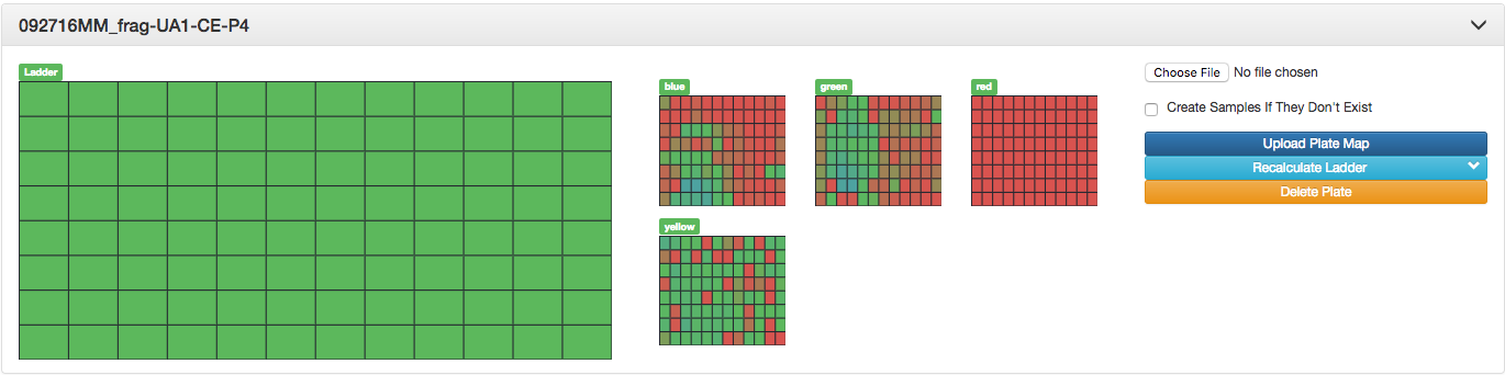
This for example shows that all ladders have been called adequately, but there appear to be some problems in the blue and green channels, indicating there were likely some issues in setting up the experiment such as not mixing well enough or inconsistent transfer of material. The red channel has no peaks identified because the ladder in this case was run in the red channel.
Projects are the primary analysis unit in MicroSPAT. They consist of a Locus Set, a set of samples to be analyzed, and the scanning, filtering, and project specific parameters for each locus. Multiple projects may reference the same samples, allowing for rapid iteration of analysis using different settings.
Bin Estimator Projects are used to create bin sets, the ranges of expected peak sizes that correspond to different alleles. After peaks are identified, a mean shift clustering algorithm is applied on the peak base size dimension to identify modes in the data, which are interpreted as alleles present.
To create a new Bin Estimator Project, select the Bin Estimators tab in the left panel. Fill in the relevant information, including a unique title and the locus set to be analyzed.
After creating a new Bin Estimator Project, select the project and navigate to the Loci tab. From here, each locus may be individually analyzed to create a new bin set. Currently, all data for a given locus available at the time of project creation is used. In the future, the user will have the option of choosing which samples to include in a Bin Estimator Project.
| Parameter | Description |
|---|---|
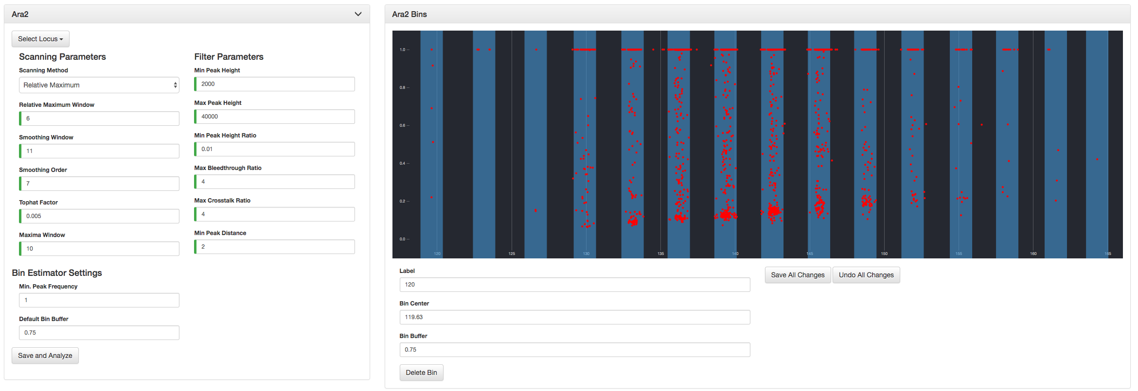
| Min. Peak Frequency | The minimum number of peaks present before a bin is created |
| Default Bin Buffer | The default bin buffer size each bin is created with |
After analysis, a view will be presented that shows where every non-filtered peak falls, the x-axis is the peak base size, the y-axis is the peak relative height (1 indicates that the peak is the primary, tallest, peak). The user at this point may manipulate the bins manually by selecting a bin and shifting the buffer size or moving the center. After changes are made, press "Save All Changes" to persist the changes to the database. Additional bins may also be added by right clicking the panel and selecting "Add Bin".
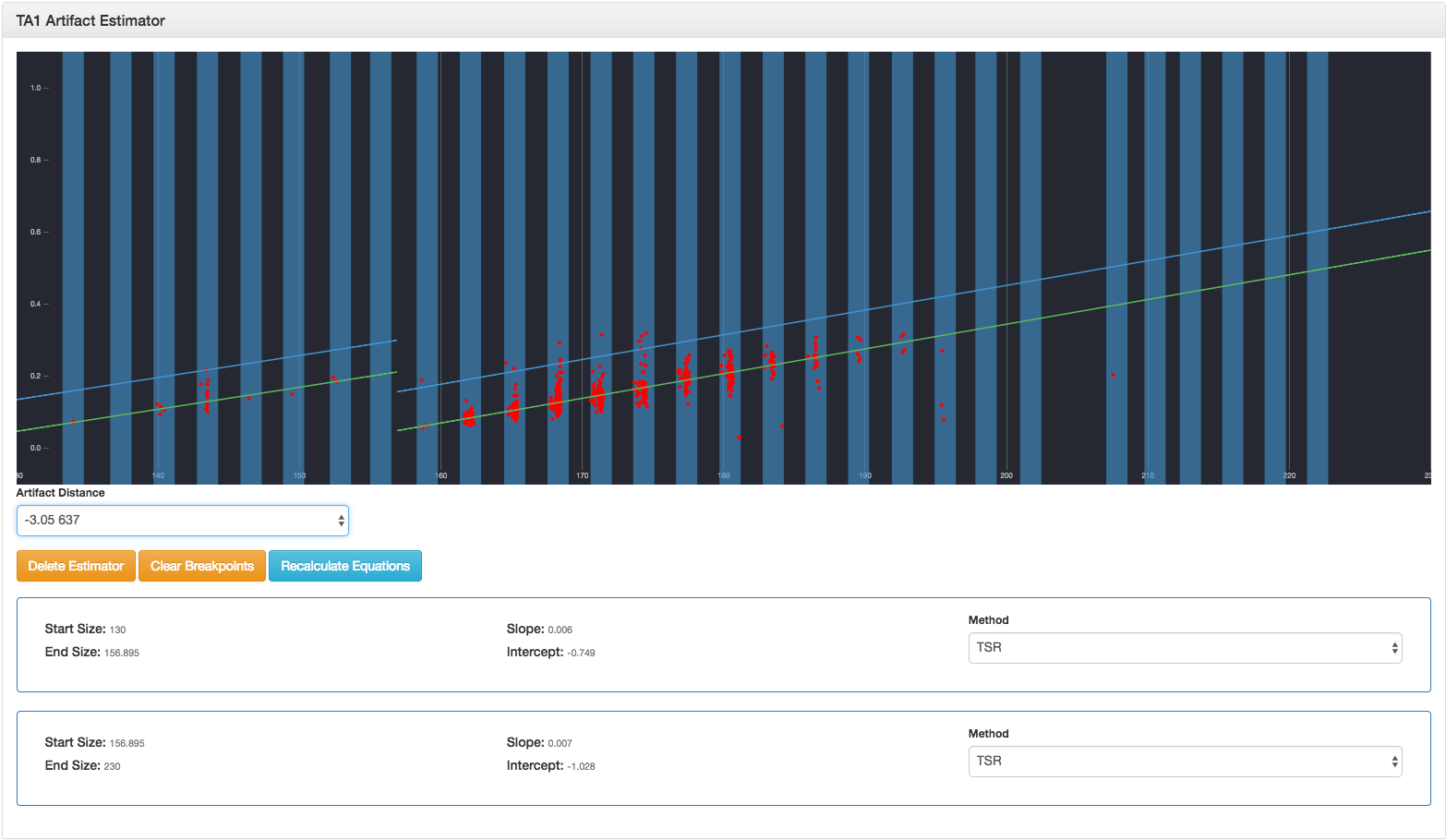
Artifact Estimator Projects are used to generate artifact estimator equations, simple linear models that predict artifact peaks. Artifact peaks are false peaks that occur consistently relative to a true peak, and their heights can be described as a function of the height of a true peak. After peaks are identified, the Artifact Estimator Project will cluster peaks based on their distance to the presumed primary true peak. Within each of these groupings, the Artifact Estimator Project will then generate a linear model that describes the relationship.
To create a new Artifact Estimator Project, select the Artifact Estimators tab in the left panel. Fill in the relevant information, including a unique title, the locus set to be analyzed, and a valid Bin Estimator Project that will be used to bin peaks.
After creating a new Arfitact Estimator Project, select the project and navigate to the Loci tab. From here, each locus may be individually analyzed to create a new Artifact Estimator Equation Set. Currently, all data for a given locus available at the time of project creation is used. In the future, the user will have the option of choosing which samples to include in a Artifact Estimator Project. During analysis, runs are only used if they are determined to be mono-allelic, that is, there is only one primary peak.
| Parameter | Description |
|---|---|
| Max Secondary Relative Peak Height | Used to determine mono-allelic runs. A run is mono-allelic if all secondary peaks have a relative peak height less than Max Secondary Relative Peak Height |
| Min Artifact Peak Frequency | Minimum number of peaks that must be present in a relative distance class before an Artifact Estimator Equation Set is generated. |
After analyzing peaks for a given locus, a set of equations are created that describe the relationship of the primary peak to the identified artifact peak classes, where each class is a discrete distance from the primary peak. Within each class, there may be one or more linear regressions that describe the relationship as a function of the base size of the primary peak. There are 4 main methods for generating linear regressions:
| Method | Description |
|---|---|
| Least Squares Regression (LSR) | Minimizes the residual sum of squares between observed response and response predicted |
| Theil-Sen Regression (TSR) | Non-parametric method, median-based estimator that is more robust to outliers. Default estimator used |
| Random Sampling Consensus (RANSAC) | Iterative algorithm that is robust to outliers. Partitions peaks into inliers and outliers, uses only inliers to generate model. Provides very tight estimates of artifact, however is erratic when little data is available |
| No Slope | Estimate is the mean of the data |
Quantification Bias Estimator Projects are used to estimate the original proportion of DNA in a sample contributed by a particular allele. In runs where the peak height does not exceed the offscale threshold, it is possible to use the peak height as a proxy for the original proportion of DNA that is made up by a particular allele. However, amplification dynamics during PCR cause shorter alleles to be preferentially amplified, causing their peak signal intensity to be overrepresented. This preferential amplification can be corrected for by a Quantification Bias Estimator Project. Given a set of samples containing two unique sets of DNA in known proportions, the Quantification Bias Estimator Project can determine the characteristic amplification bias for a locus as function of the base size difference between alleles.
To create a new Quantification Bias Estimator Project, select the Quantification Bias Estimators tab in the left panel. Fill in the relevant information, including a unique title, the locus set to be analyzed, a valid Bin Estimator Project that will be used to identify valid controls, and optionally an Artifact Estimator Project to remove artifact contribution from peak height for a potentially more accurate Quantification Bias Estimator.
Prior to creating a Quantification Bias Estimator Project, controls must be established. Refer to the Controls section. To assign samples to the project, select the Samples tab and upload a CSV containing the unique barcode of the sample, as well as the relative proportion of controls contained in the sample. The header will be [Barcode, C1, C2, ...] where the columns following Barcode indicate a unique control contained within the sample. Each row then contains the barcode of the sample that has been assigned to wells in plates, and each cell following contains the unique label of a Control (as established under the controls section), and its respective proportion, delimited by a semicolon. Ex:
| Barcode | C1 | C2 |
|---|---|---|
| MIXC-DS1-DC1 | V1S;0.5 | U659;0.5 |
| ... | ... | ... |
The proportions of each strain must add up to 1. A demonstration file may be found in demo_files\control_samples.csv
After creating a new Quantification Bias Estimator Project and assigning Control samples, navigate to the Loci tab. From here, each locus may be individually analyzed to determine the Quantification Bias Factor that can be used to correct for amplification bias.
| Parameter | Description |
|---|---|
| Min Peak Height | Minimum peak height for the peak to be included in estimation |
| Min True Peak Proportion | Minimum proportion an allele must contribute for it to be included in Quantification Bias Factor estimation (also excludes anything greater than 1 - min true peak proportion) |
| Offscale Threshold | Maximum peak height before a run is discarded because the peak height will not be representative of original DNA composition |
Genotyping Projects are used to determine the alleles present in unknown samples. When combined with only a Bin Estimator, functionality is similar to Genemapper, allowing for rapid parameterized peak identification and binning that can be manually reviewed. When also combined with an Artifact Estimator, peak identification becomes much more nuanced, allowing for much improved artifact peak identification and resolution of low density populations.
To create a new Genotyping Project, select the Genotyping Projects tab in the left panel. Fill in the relevant information, including a unique title, the locus set to be analyzed, a valid Bin Estimator Project that will be used to bin peaks, optionally an Artifact Estimator Project to aid in identifying artifact peaks, and also optionally a Quantification Bias Estimator Project to get a more accurate relative quantification of alleles, allowing for potential phasing of haplotypes in mixed populations.
After creating a Genotyping Project, navigate to the Samples tab. To add samples to the project, upload a CSV file with a header of [Barcode], and each row is the unique barcode of the sample to be analyzed. The sample must exist in the database prior to this, such as when samples are added during Plate Map assignment. After samples are added, the list below will populate with the sample barcodes.
After creating a new Genotyping Project and adding Samples, navigate to the Loci tab. From here, each locus may be individually analyzed to determine the alleles present in each sample at the particular locus.
| Parameter | Description |
|---|---|
| Min Relative Peak Height | Peaks with a height relative to the tallest peak that do not exceed Min Relative Peak Height are classified as artifact |
| Min Absolute Peak Height | Minimum peak height for a peak to not be classified as artifact |
| Bleedthrough Limit | Maximum bleedthrough ratio before a peak is classified as bleedthrough |
| Crosstalk Limit | Maximum crosstalk ratio before a peak is classified as crosstalk |
| Failure Threshold | At least one peak's height must exceed the failure threshold, otherwise the run is deemed a failure and rejected |
| Soft Artifact SD Limit | Peaks with a height that falls within the Soft Artifact SD Limit times the artifact error plus the estimated artifact contribution have a peak probability calculated when probabilistic annotation is enabled |
| Hard Artifact SD Limit | Peaks with a height minus (artifact contribution + artifact error * Hard Artifact SD Limit) < Min Absolute Peak Height are classified as artifact |
| Genotyping Probability Threshold | Peaks with a probability less than the Genotyping Probability Threshold are classified as artifact |
| Bootstrap Probability Threshold | Peaks with a probability less than the Bootstrap Probability Threshold are culled during the iterative peak frequency and sample MOI estimation steps during probabilistic peak annotation |
| Offscale Threshold | Runs with a peak that exceeds the Offscale Threshold are flagged as offscale and are avoided if possible |